ID: 31237266 MATIAS FIGUEIRAS
“I am aware of the requirements of good academic practice and the potential penalties for any breaches”.
INTRODUCTION
This blog aims are to investigate and discuss the behaviour of three different elastic materials, in their elastic and plastic regions, and experimentally verify the validity of Hooke’s Law.
THEORY
In the 17th century, physicist Robert Hooke published the law that is named after him. Hooke’s Law states that “The stress vs strain curve for many materials has a linear region. Within certain limits, the force required to stretch an elastic object such as a metal spring is directly proportional to the extension of the spring” 1.
This relationship can be expressed as follows:
F = k∆L (1)
Where F is the force, ∆L is the length of extension/compression of the material and the constant k is sometimes called the mechanical stiffness and has the units of Newtons per metre (Nm-1). If we are talking about a spring, k is called the “spring constant”.
Equation 1 can also be expressed sometimes with a minus (-) sign before the mechanical stiffness constant. This is to represent that the restoring force, due to the material/object (e.g. Spring), is in the opposite direction to the force that caused the deformation. In other words, “pulling down on a spring will cause an extension of the spring downward, which will result in an upward force due to the spring” 1.
Following Hooke’s Law, if the amount of mass hanging from the material is doubled, the length that the material stretches should also be doubled.

It is important to notice that if the material continues to be stretched, it will stop obeying Hooke’s Law after some point.

The point on the graph where it stops obeying Hooke’s Law is often called the ‘limit of proportionality’. At this point, the material has been permanently deformed.
METHOD

Figure 3 shows an ideal setup for testing the law of elasticity. The spring in this diagram represents the three different materials tested. The materials were clamped to the top of the stand and the known masses were added gently to the bottom end. First, the length of the material was registered without any mass, and later masses were added one at a time while the difference in length was recorded. All measurement was taken only once the material had stopped moving and settled in position, and the ruler was fixed at the beginning and not moved throughout the experiment. The data was later plotted in different graphs to be evaluated.
DATA GATHERED AND INTERPRETATION OF RESULTS
Testing of Materials 1 and 2

Table 1. shows the data obtained for Material 1 and 2. The y-values for Material 2 were calculated using Excel, with the following equation:
y2 = (a+0.5)x+c (2)
Where a is the gradient of the trend line for the force versus deformation graph for Material 1 and c was 0.2 (arbitrary value).
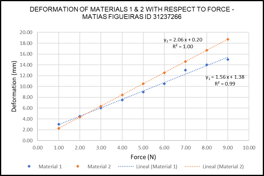
Chart 1 shows the relationship between the force applied and the deformation for Material 1 and 2.
The results agree with Hooke’s Law, as they show a linear relationship between the force applied and the change in length for both materials. This observation is supported by the R2 coefficient for each material, which in both cases is above or equal to 0.99.
“The R2 coefficient of determination is a statistical measure of how well the regression predictions approximate the real data points. An R2 of 1 indicates that the regression predictions perfectly fit the data” 5.
Owing to this linear relationship, the values for k (mechanical stiffness) can be obtained from the graph.
From equation (1), the value of k is:
k = ∆F/∆L (3)
And the gradient (m) for Graph 1 is calculated by:
m = ∆L/∆F (4)
So, the values for k can be found as the inverse of m:
k = 1/m (5)
For Material 1 k1 = 1/0.00156 = 641.03 Nm-1 & Material 2: k2 = 1/0.00206 = 485.44 Nm-1
As is clearly visible from Graph 1, Material 2 extended more than Material 1 under the same force. This is explained by the lower value for the mechanical stiffness of Material 2 ( k2).
Graph 1 also shows the point at which both materials experimented equal deformation when the same force was applied. The visual estimation for this point is (2.35;5).
Mathematically, this condition occurs when y1 = y2
From Graph 1: 1.56x+1.38 = 2.06x+0.20 –> 0.5x = 1.18 –> x = 2.36
y1 = 1.562.36+1.38 –> y = 5.06
This means that both Materials had a deformation of 5.06mm when a force of 2.36N was applied.
Testing after the elastic limit

Table 2 shows the data obtained for Material 3. The z-values for Material 2 were calculated using Excel, with the following equation:
z= x3+b (2)
Where b is the y-intercept value of the trend line for the force versus deformation graph for Material 1.
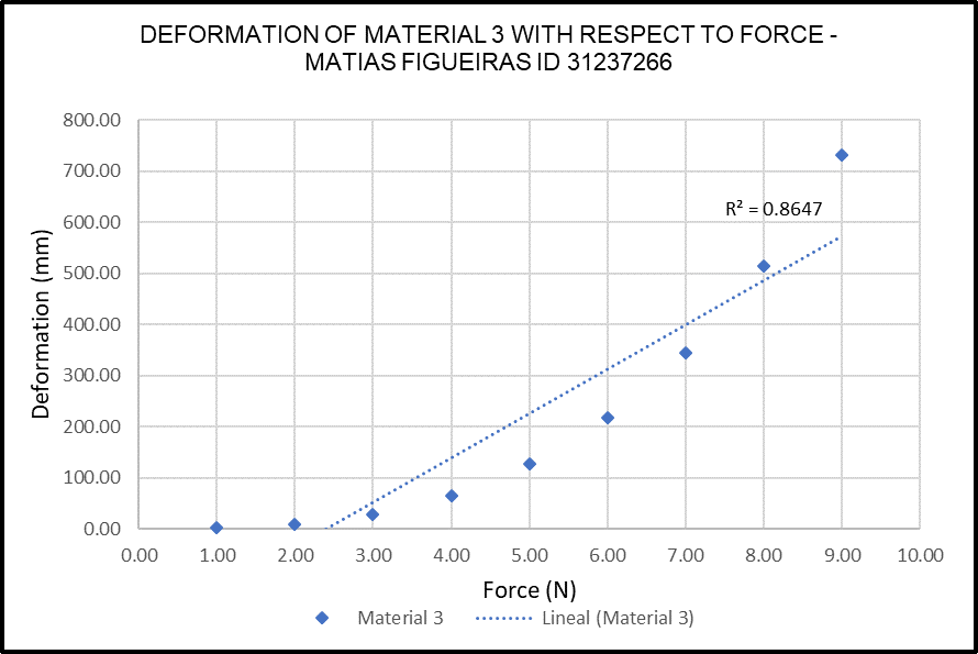
Chart 2 shows the relationship between the force applied and deformation for Material 3. As this chart clearly shows, the relationship is far from linear. If a linear trend line is applied to the data, the resulting R2 coefficient is less than 0.99, which confirms that the relationship is not linear, but rather exponential.
These results do not agree with Hooke’s Law, as the mechanical stiffness (k) at different intervals is different. This type of behaviour shows that Material 3 has gone under plastic deformation, caused by a force higher than the elastic limit of the material.
CONCLUSIONS
This experiment proves that Hooke’s Law statement is valid. The deformation is directly proportional to the force, given that the force is in the elastic limit.
Material 1 and 2 are still in their elastic regions because their extension was proportional to the force acting on them. This means that once the force is removed, they will return to their original length. It can also be said that Material 2 is more elastic than material 1 because it presents a smaller k.
Material 3 has passed its elastic limit and is said to be in its plastic region. In this case, the material will not return to its original shape after the force is removed.
The principal sources of error for this experiment are as follows:
- Many calculations depend on the previous one, so rounding errors can be present.
- The deformation is small and therefore can be easily misread when the ruler is used. This can be solved by using a more accurate instrument or by taking a picture of the reading and zooming in.
REFERENCES
[1]. https://www.khanacademy.org/science/physics/work-and-energy/hookes-law/a/what-is-hookes-law
[2]. http://xaktly.com/HookesLaw.html
[3]. https://www.khanacademy.org/science/physics/work-and-energy/hookes-law/a/what-is-hookes-law
[4]. https://www.khanacademy.org/science/physics/work-and-energy/hookes-law/a/what-is-hookes-law
[5]. https://www.khanacademy.org/science/physics/work-and-energy/hookes-law/a/what-is-hookes-law
